Inverse Relationship

Definition of Inverse Relationship

Inverse relationship is a type of correlation that exists between two variables wherein an increase in one variable is associated with a decrease in another variable. 

In other words, an inverse relationship, also known as negative relationship, is a contrary correlation between two variables such that they move in opposite directions.

For example, we have two variables X and Y. As X increases, Y decreases and as Y increases, X decreases.

In statistics, an inverse relationship or correlation is denoted by the correlation coefficient “r” having a value between -1 and 0, with r= -1 indicating perfect inverse correlation.

Another common example for this type of relationship is between interest rates and consumer spending.

When the interest rates increase, consumers are less willing to spend and more willing to save. In addition, when unemployment increases, consumer spending decreases because people have less disposable income.

Definition of Correlation

Correlation is a statistic that measures the degree to which two variables move in relation to each other. It shows the strength of a relationship between two variables and is expressed numerically by the correlation coefficient (r).

Inverse Correlation Graph

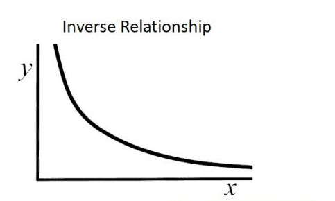
Two sets of data points can be plotted on a graph on an x and y-axis to check for correlation. This is called a scatter diagram, which represents a visual way to check for a positive or negative correlation.

The graph below shows a strong negative relationship between two sets of data points plotted on the graph.

Example of Calculating Inverse Correlation

Correlation can be calculated between two sets of data to arrive at a numerical result. The resulting statistic is used in a predictive manner to estimate metrics like the risk reduction benefits of portfolio diversification and other important data.

The example presented below shows how to calculate the statistic.

Assume an analyst needs to calculate the degree of correlation between the following two data sets:

• X: 10, 8, 7, 5, 3
• Y: 2, 5, 6, 8, 9

There are three steps involved in finding the correlation. First, add up all the X values to find SUM(X), add up all the Y values to find SUM(Y) and multiply each X value with its corresponding Y value and sum them to find SUM(X,Y):

SUM(X) = 10 + 8 + 7 + 5 + 3

= 33

SUM(Y) = 2 + 5 + 6 + 8 + 9

= 30

SUM(X,Y) = (10X2) + (8X5) + (7×6) + (5X8) + (3X9)

= 169

The next step is to take each X value, square it and sum up all these values to find SUM(X²). The same must be done for the Y values:

SUM(X²) = (10²) + (8²) + (7²) + (5²) + (3²)

= 247

SUM (Y²) = (2²) + (5²) + (6²) + (8²) + (9²)

= 210

Noting there are five observations, n, the following formula can be used to find the correlation coefficient, r:

$$r=\dfrac{[n\:x\:(SUM(X,Y)-(SUM(X)\:x\:(SUM(Y))]}{[(n\:x\:SUM(X^2)-SUM(X)^2]\:x\:[nxSUM(Y^2)-SUM(y)^2)]}$$

In this example, the correlation is:

• r =   –145

       911

• r = –0.159 

The two data sets have a correlation of –0.159, which is called an inverse correlation because it is a negative number.

Inverse Relationships in Economics

There are many instances of inverse relationships in economics. 

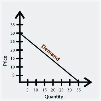
The one most common encountered is the price-demand relationship, where quantity demanded falls (rises) as price increases (decreases). This relationship is widely known as the law of demand.

The demand curve shows the quantity demanded of a product at different price levels.

Kindly note that demand is not the same thing as quantity demanded.

Demand for a good depends on many factors such as, the price of the good and that of other goods, the level of income and wealth, individual preferences, etc. The demand curve above shows the quantities of the good demanded at different price levels, when the other factors are held constant.

The inverse correlation between the price of the good and its quantity demanded depends on two factors:

1. Reduction in price. It means more goods can be purchased for the same expenditure as before.
2. Lower price of one product increases real income, since less money is needed to purchase the product, even though money income remains the same. An increase in real income means that more of all goods, including the one whose price has been reduced, can be purchased.

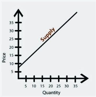
By contrast, the supply curve illustrates a direct relationship.

When prices go up, existing suppliers will try to sell more, while new suppliers will be encouraged to enter the market. As a result, the quantity supplied of the product will increase as prices rise.

Inverse Relationships in Finance

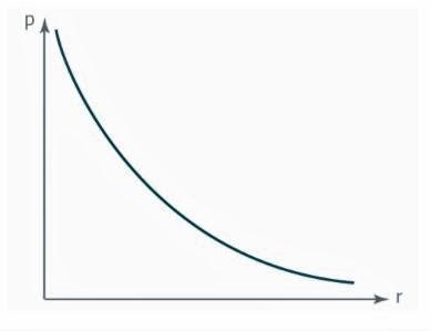
There is an inverse relationship between interest rates and bond prices.

Bond is a fixed income financial instrument. Thus, bond prices fall as interest rates go up and rise as interest rates go down.

When a bond is issued, its face value, which is the amount of money, usually $1,000, the bond was issued to raise, is set. In addition, the bond will carry a coupon rate, which determines the fixed coupon payment. Thus a 10% coupon rate means that the $1,000 bond will pay $100 annually.

If a $1,000 bond of similar risk is issued that has a coupon rate of 12%, the 10% bonds will fall in value, because they pay only $100 annually, when the new bonds are paying $120. The price of the old bonds will fall until their $100 per annum payout equals 12%, i.e., $100/0.12 = $833.33.

This inverse correlation between bond prices and interest rates can be plotted on a graph, as above.

Inverse Relationships in Math

In math, we often come across pairs of variables that are linked in some way.

For example, a data set shows: {(-6, -7) (-4, -3) (1, 5) (3, 7)},

where the values that occur first represent one variable and the values in second position represent another variable.

In many cases, the values representing the first variable may be represented as the X-values and those representing the second variable, as Y-values.

The connection between the two variables may depend on some causal relationship or they may have been paired randomly. Regardless, by virtue of being paired, the X and Y values in each pair, and by extension, the two variables which they represent are now in a relationship.

That relationship may be described by a rule that takes the values of the first variable (X-values) and tells us the corresponding values of the second variable (Y-values).

Just as reasonably, the relationship may be described by a rule that takes the values of the second variable (Y-values) and tells us the corresponding values of the first variable (X-values). Such rules in mathematics are known as functions.

A mathematical function is simply a rule that describes the relationship between ordered pairs, going either from X-values to Y-values, in which case it is written Y = f(X) or from Y-values to X-values and written X = f(Y) or Y = f^-1(X).

The set of values of the variable in brackets is called the domain, while the set of values of the other variable is known as the range. Thus, in Y = f(X), the X-values are the domain, while the Y-values are the range.

Sometimes, a function is described as a machine that takes input – the X-values – and delivers output – the Y-values.

As with any rule, its outcome must be definite. It means a rule should give the same result today and tomorrow. Accordingly, in f = (X), any X-value must result in only one Y-value and all X-values must have a result.

Hence, for any set of ordered pairs, there will be two rules, with one being the inverse of the other, i.e., the second rule would have described a function that is the inverse of the first rule. And the second function would bear an inverse relationship to the first function.

Inverse as Opposite of Direct Relationship

However, an inverse relationship may also exist between the X and Y variables rather than the functions. In such cases, an inverse relationship is the opposite of a direct relationship, where in Y = f(X), Y increases as X increases or in X = f(Y), X increases as Y increases.

In an inverse relationship, given by Y = f(X), Y would decrease as X increases.

More Examples of Inverse Relationship

There are many real-life examples of inverse relationships.

• Travel speed and travel time. The faster one travels from point A to point B; the less travel time is required to arrive at point B from point A.
• Current and resistance. The higher the resistance, the lower the current.
• Savings and disposable income.  The less the disposable income, the more the savings.
• Government spending and unemployment rate. The higher the government spending, the lower the unemployment rate.
• Unemployment rate and inflation, also known as the Phillips Curve.

The Phillips Curve is the most common example of inverse relationship.

It is an economic concept developed by A.W. Phillips stating that inflation and unemployment rate have a stable and inverse relationship. The theory claims that with economic growth comes inflation, which in turn should lead to more jobs and less unemployment.

In reality, when the government spending increases, the unemployment rate decreases because more jobs are created. Following the higher government spending, employees are better compensated, which means that they have more money to spend.

On the other hand, firms face higher compensation costs, which are passed to consumers through inflation. Hence, the lower the unemployment rate, the higher the inflation.

Brief Summary About Phillips Curve

Since the Phillips curves suggests there is an inverse relationship between inflation and unemployment, policymakers then have an option on what to prioritize between the two. 

During the 1950s and 1960s, Phillips curve analysis suggested there was a trade-off, and policymakers could use demand management (fiscal and monetary policy) to try and impact the rate of economic growth and inflation. Which means, if unemployment was high and inflation low, policymakers could stimulate aggregate demand. This would aid to reduce unemployment, but cause a higher rate of inflation.

In the 1970s however, there seemed to be a breakdown in the Phillips curve when stagflation (higher unemployment and higher inflation) occurred. The Phillips Curve was then criticized by monetarist economists who argued there was no trade-off between unemployment and inflation in the long run.

Regardless, some feel that the Phillips Curve still has some relevance and policymakers still need to consider the potential trade-off between unemployment and inflation.

Relevance of Phillips Curve Today

In the current economic climate, many Central Banks and policymakers are weighing up how much importance they should give to reducing unemployment and inflation. For example, the Federal Reserve is considering using monetary policy to achieve an unemployment target and a willingness to accept higher inflation.

During 2009-13, the Bank of England has been willing to tolerate inflation above the government’s target of 2% because they feel to reduce inflation would have caused serious problems for unemployment and economic growth.

This willingness to consider a higher inflation rate, suggest policymakers feel that the trade-off of higher inflation is worth the benefit of lower unemployment. However, not all economists agree we should be allowing the inflation target to increase.

If we allow inflation to increase, inflationary pressures will become engrained, and monetary policy will lose credibility. 

What Does Inverse Correlation Tell You?

Inverse correlation tells you that when one variable increases, the other tends to decrease.

Two points need to be kept in mind with regard to inverse or negative correlation:

First, the existence of a negative correlation, or positive correlation for that matter, does not necessarily imply an underlying relationship.

Second, the relationship between two variables is not static and fluctuates over time. It means the variables may show an inverse correlation during some periods and a positive correlation during others.

Limitations of Using Inverse Correlation

Correlation analysis can tell useful information about the relationship between two variables, such as how the stock and bond markets often move in opposite directions. However, the analysis does not fully consider outliers or unusual behavior of a few data points within a given set of data points, which could twist the outcomes.

Similarly, when two variables show an inverse correlation, there might be some other variables that, while not part in the study, do in fact affect the variable in question. Even though two variables have a very strong inverse correlation, this result never implies a cause and effect relationship between the two.

Finally, using the results of a correlation analysis to infer the same conclusion to new data carries a high degree of risk.